- Scikit Learn - Home
- Scikit Learn - Introduction
- Scikit Learn - Modelling Process
- Scikit Learn - Data Representation
- Scikit Learn - Estimator API
- Scikit Learn - Conventions
- Scikit Learn - Linear Modeling
- Scikit Learn - Extended Linear Modeling
- Stochastic Gradient Descent
- Scikit Learn - Support Vector Machines
- Scikit Learn - Anomaly Detection
- Scikit Learn - K-Nearest Neighbors
- Scikit Learn - KNN Learning
- Classification with Naïve Bayes
- Scikit Learn - Decision Trees
- Randomized Decision Trees
- Scikit Learn - Boosting Methods
- Scikit Learn - Clustering Methods
- Clustering Performance Evaluation
- Dimensionality Reduction using PCA
- Scikit Learn Useful Resources
- Scikit Learn - Quick Guide
- Scikit Learn - Useful Resources
- Scikit Learn - Discussion
Scikit Learn - KNeighborsClassifier
The K in the name of this classifier represents the k nearest neighbors, where k is an integer value specified by the user. Hence as the name suggests, this classifier implements learning based on the k nearest neighbors. The choice of the value of k is dependent on data. Lets understand it more with the help if an implementation example −
Implementation Example
In this example, we will be implementing KNN on data set named Iris Flower data set by using scikit-learn KneighborsClassifer.
This data set has 50 samples for each different species (setosa, versicolor, virginica) of iris flower i.e. total of 150 samples.
For each sample, we have 4 features named sepal length, sepal width, petal length, petal width)
First, import the dataset and print the features names as follows −
from sklearn.datasets import load_iris
iris = load_iris()
print(iris.feature_names)
Output
['sepal length (cm)', 'sepal width (cm)', 'petal length (cm)', 'petal width (cm)']
Example
Now we can print target i.e the integers representing the different species. Here 0 = setos, 1 = versicolor and 2 = virginica.
print(iris.target)
Output
[
   0 0 0 0 0 0 0 0 0 0 0 0 0 0 0 0 0 0 0 0 0 0 0 0 0 0 0 0 0 0 0 0 0 0 0 0 0
   0 0 0 0 0 0 0 0 0 0 0 0 0 1 1 1 1 1 1 1 1 1 1 1 1 1 1 1 1 1 1 1 1 1 1 1 1
   1 1 1 1 1 1 1 1 1 1 1 1 1 1 1 1 1 1 1 1 1 1 1 1 1 1 2 2 2 2 2 2 2 2 2 2 2
   2 2 2 2 2 2 2 2 2 2 2 2 2 2 2 2 2 2 2 2 2 2 2 2 2 2 2 2 2 2 2 2 2 2 2 2 2
   2 2
]
Example
Following line of code will show the names of the target −
print(iris.target_names)
Output
['setosa' 'versicolor' 'virginica']
Example
We can check the number of observations and features with the help of following line of code (iris data set has 150 observations and 4 features)
print(iris.data.shape)
Output
(150, 4)
Now, we need to split the data into training and testing data. We will be using Sklearn train_test_split function to split the data into the ratio of 70 (training data) and 30 (testing data) −
X = iris.data[:, :4]
y = iris.target
from sklearn.model_selection import train_test_split
X_train, X_test, y_train, y_test = train_test_split(X, y, test_size = 0.30)
Next, we will be doing data scaling with the help of Sklearn preprocessing module as follows −
from sklearn.preprocessing import StandardScaler
scaler = StandardScaler()
scaler.fit(X_train)
X_train = scaler.transform(X_train)
X_test = scaler.transform(X_test)
Example
Following line of codes will give you the shape of train and test objects −
print(X_train.shape)
print(X_test.shape)
Output
(105, 4)
(45, 4)
Example
Following line of codes will give you the shape of new y object −
print(y_train.shape)
print(y_test.shape)
Output
(105,)
(45,)
Next, import the KneighborsClassifier class from Sklearn as follows −
from sklearn.neighbors import KNeighborsClassifier
To check accuracy, we need to import Metrics model as follows −
from sklearn import metrics
We are going to run it for k = 1 to 15 and will be recording testing accuracy, plotting it, showing confusion matrix and classification report:
Range_k = range(1,15)
scores = {}
scores_list = []
for k in range_k:
   classifier = KNeighborsClassifier(n_neighbors=k)
   classifier.fit(X_train, y_train)
   y_pred = classifier.predict(X_test)
   scores[k] = metrics.accuracy_score(y_test,y_pred)
   scores_list.append(metrics.accuracy_score(y_test,y_pred))
result = metrics.confusion_matrix(y_test, y_pred)
print("Confusion Matrix:")
print(result)
result1 = metrics.classification_report(y_test, y_pred)
print("Classification Report:",)
print (result1)
Example
Now, we will be plotting the relationship between the values of K and the corresponding testing accuracy. It will be done using matplotlib library.
%matplotlib inline
import matplotlib.pyplot as plt
plt.plot(k_range,scores_list)
plt.xlabel("Value of K")
plt.ylabel("Accuracy")
Output
Confusion Matrix:
[
   [15 0 0]
   [ 0 15 0]
   [ 0 1 14]
]
Classification Report:
            precision   recall   f1-score    support
         0     1.00     1.00        1.00        15
         1     0.94     1.00        0.97        15
         2     1.00     0.93        0.97        15

micro avg      0.98     0.98        0.98        45
macro avg      0.98     0.98        0.98        45
weighted avg   0.98     0.98        0.98        45

Text(0, 0.5, 'Accuracy')
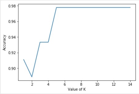
Example
For the above model, we can choose the optimal value of K (any value between 6 to 14, as the accuracy is highest for this range) as 8 and retrain the model as follows −
classifier = KNeighborsClassifier(n_neighbors = 8)
classifier.fit(X_train, y_train)
Output
KNeighborsClassifier(
   algorithm = 'auto', leaf_size = 30, metric = 'minkowski',
   metric_params = None, n_jobs = None, n_neighbors = 8, p = 2,
   weights = 'uniform'
)
classes = {0:'setosa',1:'versicolor',2:'virginicia'}
x_new = [[1,1,1,1],[4,3,1.3,0.2]]
y_predict = rnc.predict(x_new)
print(classes[y_predict[0]])
print(classes[y_predict[1]])
Output
virginicia
virginicia
Complete working/executable program
from sklearn.datasets import load_iris
iris = load_iris()
print(iris.target_names)
print(iris.data.shape)
X = iris.data[:, :4]
y = iris.target

from sklearn.model_selection import train_test_split
X_train, X_test, y_train, y_test = train_test_split(X, y, test_size=0.30)

from sklearn.preprocessing import StandardScaler
scaler = StandardScaler()
scaler.fit(X_train)
X_train = scaler.transform(X_train)
X_test = scaler.transform(X_test)

print(X_train.shape)
print(X_test.shape)

from sklearn.neighbors import KNeighborsClassifier

from sklearn import metrics

Range_k = range(1,15)
scores = {}
scores_list = []
for k in range_k:
   classifier = KNeighborsClassifier(n_neighbors=k)
   classifier.fit(X_train, y_train)
   y_pred = classifier.predict(X_test)
   scores[k] = metrics.accuracy_score(y_test,y_pred)
   scores_list.append(metrics.accuracy_score(y_test,y_pred))
result = metrics.confusion_matrix(y_test, y_pred)
print("Confusion Matrix:")
print(result)
result1 = metrics.classification_report(y_test, y_pred)
print("Classification Report:",)
print (result1)
%matplotlib inline
import matplotlib.pyplot as plt
plt.plot(k_range,scores_list)
plt.xlabel("Value of K")
plt.ylabel("Accuracy")

classifier = KNeighborsClassifier(n_neighbors=8)
classifier.fit(X_train, y_train)

classes = {0:'setosa',1:'versicolor',2:'virginicia'}
x_new = [[1,1,1,1],[4,3,1.3,0.2]]
y_predict = rnc.predict(x_new)
print(classes[y_predict[0]])
print(classes[y_predict[1]])