
 Data Structure
 Networking
 RDBMS
RDBMS Operating System
 Java
Java MS Excel
 iOS
iOS HTML
HTML CSS
CSS Android
 Python
 C Programming
 C++
C++ C#
C# MongoDB
 MySQL
MySQL Javascript
 PHP
PHP
- Selected Reading
- UPSC IAS Exams Notes
- Developer's Best Practices
- Questions and Answers
- Effective Resume Writing
- HR Interview Questions
- Computer Glossary
- Who is Who
Plotting graph For IRIS Dataset Using Seaborn And Matplotlib
The Iris dataset is a widely recognized benchmark in data analysis and visualization using matplotlib and seaborn which are libraries of Python. This article presents a comprehensive guide on how to plot graphs for the Iris dataset using two powerful Python libraries: Seaborn and Matplotlib. Leveraging Seaborn's built-in Iris dataset, we explore the step-by-step process of loading the data, performing data preprocessing, and conducting insightful data analysis.
With the help of Seaborn's pairplot function, we create visually appealing scatter plots that showcase the relationships between different features and the distinct species of Iris flowers. By following this tutorial, readers will gain practical knowledge in visualizing and interpreting the Iris dataset effectively.
How to plot graph for IRIS Dataset Using Seaborn And Matplotlib?
Below are the steps for Plotting graph For IRIS Dataset Using Seaborn And Matplotlib ?
Algorithm
We begin by importing the necessary libraries: seaborn, matplotlib.pyplot, and pandas. These libraries are commonly used for data analysis and visualization in Python.
We load the Iris dataset using the load_dataset function from Seaborn and assign it to the variable iris. The Iris dataset is a popular dataset that contains measurements of four features for three different species of Iris flowers (setosa, versicolor, and virginica).
Next, we perform data preprocessing. In this example, we separate the features and the target variable. The X = iris.drop('species', axis=1) line creates a new DataFrame X by dropping the 'species' column from the iris DataFrame. The axis=1 parameter specifies that we want to drop a column. The y = iris['species'] line assigns the 'species' column to the variable y, which represents the target variable we want to predict.
After data preprocessing, you can perform any necessary data processing steps based on your analysis requirements. This could include handling missing values, scaling the features, or any other transformations required for your analysis. This section is left blank in the example code, and you can insert your data processing steps as needed.
We then perform data analysis. In this example, we calculate the summary statistics of the features using the describe() method on the X DataFrame. We store the results in the variable summary_stats.
We print the summary statistics to the console using the print() function. This will display the summary statistics for each feature in the Iris dataset, including the count, mean, standard deviation, minimum, quartiles, and maximum values.
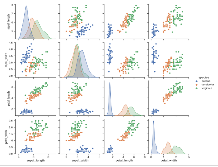
Finally, we plot the graph using Seaborn and Matplotlib. We set the Seaborn style to "ticks" using sns.set(style="ticks"). This step is optional and only affects the overall appearance of the plot. The pairplot() function from Seaborn is used to create a matrix of scatter plots, where each pair of features is plotted against each other. The iris DataFrame is passed as the data argument to pairplot(). The hue="species" parameter ensures that the points in the scatter plots are colored based on the species of Iris. This allows us to visualize the relationships between different pairs of features and observe how they are related to the different Iris species.
Finally, we use plt.show() from Matplotlib to display the graph. This will open a window or display the graph in the Jupyter Notebook or IDE where you're running the program.
By running the below program, we will perform data preprocessing, and any necessary data processing steps, calculate the summary statistics, and then generate a graph with scatter plots for the Iris dataset. The summary statistics will be printed to the console, and the graph will show the relationships between different pairs of features for the three Iris species.
Example
import seaborn as sns
import matplotlib.pyplot as plt
import pandas as pd

# Load the Iris dataset from Seaborn
iris = sns.load_dataset('iris')

# Data preprocessing
# Separate features and target variable
X = iris.drop('species', axis=1)
y = iris['species']

# Data processing
# Perform any necessary data processing steps here

# Data analysis
# Calculate summary statistics
summary_stats = X.describe()
print("Summary Statistics:")
print(summary_stats)

# Plot the graph using Seaborn and Matplotlib
sns.set(style="ticks")
sns.pairplot(iris, hue="species")
plt.show()
Output
Summary Statistics:
       sepal_length  sepal_width  petal_length  petal_width
count    150.000000   150.000000    150.000000   150.000000
mean       5.843333     3.057333      3.758000     1.199333
std        0.828066     0.435866      1.765298     0.762238
min        4.300000     2.000000      1.000000     0.100000
25%        5.100000     2.800000      1.600000     0.300000
50%        5.800000     3.000000      4.350000     1.300000
75%        6.400000     3.300000      5.100000     1.800000
max        7.900000     4.400000      6.900000     2.500000
Conclusion
In conclusion, this article has demonstrated the process of plotting graphs for the Iris dataset using Seaborn and Matplotlib. By utilizing Seaborn's pairplot function, we were able to visualize the relationships between various features and the Iris flower species.
Through data preprocessing and analysis, we gained valuable insights into the dataset. The combination of Seaborn and Matplotlib provided us with powerful tools for creating visually appealing and informative graphs.

3K+ Views
