
 Data Structure
 Networking
 RDBMS
RDBMS Operating System
 Java
Java iOS
iOS HTML
HTML CSS
CSS Android
 Python
 C Programming
 C++
C++ C#
C# MongoDB
 MySQL
MySQL Javascript
 PHP
PHPOlympics Data Analysis Using Python
The contemporary Olympic Games, sometimes known as the Olympics, are major international sporting events that feature summer and winter sports contests in which thousands of participants from all over the world compete in a range of disciplines. With over 200 nations competing, the Olympic Games are regarded as the world's premier sporting event. In this article, we will examine the Olympics using Python. Let's begin.
Importing necessary libraries
!pip install pandas
!pip install numpy
import numpy as np
import pandas as pd
import seaborn as sns
from matplotlib import pyplot as plt
Importing and understanding the dataset
We have two CSV files when dealing with Olympic data. One detailing the total sports-related expenses of all Olympic Games. Another has information on athletes from all years who competed with information.
You can get a CSV data file by clicking here ?
data = pd.read_csv('/content/sample_data/athlete_events.csv')
# data.head() display first 5 entry
print(data.head(), data.describe(), data.info())
Merging both datasets
# regions and country noc data CSV file
regions = pd.read_csv('/content/sample_data/datasets_31029_40943_noc_regions.csv')
print(regions.head())
# merging to data and regions frame
merged = pd.merge(data, regions, on='NOC', how='left')
print(merged.head())
From here the data analysis starts.
Data analysis of Gold analysis
Example
#creating goldmedal dataframes
goldMedals = merged[(merged.Medal == 'Gold')]
print(goldMedals.head())
Output
 ID                     Name    Sex   Age  Height  Weight            Team  \
3    4     Edgar Lindenau Aabye   M  34.0     NaN     NaN  Denmark/Sweden
42  17  Paavo Johannes Aaltonen   M  28.0   175.0    64.0         Finland
44  17  Paavo Johannes Aaltonen   M  28.0   175.0    64.0         Finland
48  17  Paavo Johannes Aaltonen   M  28.0   175.0    64.0         Finland
60  20       Kjetil Andr Aamodt   M  20.0   176.0    85.0          Norway

    NOC        Games  Year  Season         City          Sport  \
3   DEN  1900 Summer  1900  Summer        Paris     Tug-Of-War
42  FIN  1948 Summer  1948  Summer       London     Gymnastics
44  FIN  1948 Summer  1948  Summer       London     Gymnastics
48  FIN  1948 Summer  1948  Summer       London     Gymnastics
60  NOR  1992 Winter  1992  Winter  Albertville  Alpine Skiing

                               Event Medal   region notes
3        Tug-Of-War Men's Tug-Of-War  Gold  Denmark   NaN
42  Gymnastics Men's Team All-Around  Gold  Finland   NaN
44      Gymnastics Men's Horse Vault  Gold  Finland   NaN
48  Gymnastics Men's Pommelled Horse  Gold  Finland   NaN
60       Alpine Skiing Men's Super G  Gold   Norway   NaN
Analysis of gold medalists according to age
Here, we'll make a graph showing the number of gold medals in relation to age. For this, we will develop a counterplot for graph representation, with the participants' ages shown on the X-axis and the number of medals on the Y-axis.
Example
plt.figure(figsize=(20, 10))
plt.title('Distribution of Gold Medals')
sns.countplot(goldMedals['Age'])
plt.show()
Output

Make a new data frame named ?masterDisciplines' in which to place this new group of people. Then, use that data frame to make a visualization.
Example
masterDisciplines = goldMedals['Sport'][goldMedals['Age'] > 50]
plt.figure(figsize=(20, 10))
plt.tight_layout()
sns.countplot(masterDisciplines)
plt.title('Gold Medals for Athletes Over 50')
plt.show()
Output

Analysis women won the medals
Example
womenInOlympics = merged[(merged.Sex == 'F') &
                         (merged.Season == 'Summer')]
print(womenInOlympics.head(10))

sns.set(style="darkgrid")
plt.figure(figsize=(20, 10))
sns.countplot(x='Year', data=womenInOlympics)
plt.title('Women medals per edition of the Games')
plt.show()
Output

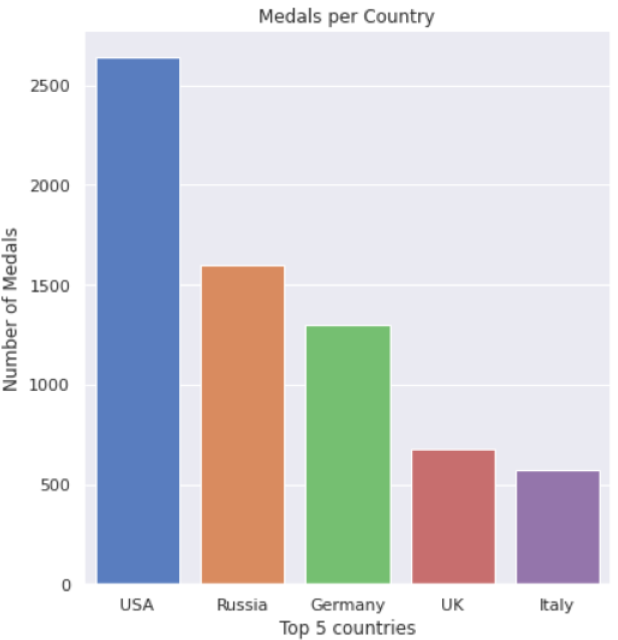
Analyzing the top 5 countries that won the medal
Example
print(goldMedals.region.value_counts().reset_index(name='Medal').head())

totalGoldMedals = goldMedals.region.value_counts().reset_index(name='Medal').head(5)
g = sns.catplot(x="index", y="Medal", data=totalGoldMedals,
                height=6, kind="bar", palette="muted")
g.despine(left=True)
g.set_xlabels("Top 5 countries")
g.set_ylabels("Number of Medals")
plt.title('Medals per Country')
plt.show()
Output
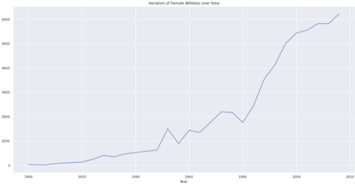
Evolution of athletes over time
Example
MenOverTime = merged[(merged.Sex == 'M') & (merged.Season == 'Summer')]
WomenOverTime = merged[(merged.Sex == 'F') & (merged.Season == 'Summer')]
part = MenOverTime.groupby('Year')['Sex'].value_counts()
plt.figure(figsize=(20, 10))
part.loc[:,'M'].plot()
plt.title('Variation of Male Athletes over time')
Output

Example
part = WomenOverTime.groupby('Year')['Sex'].value_counts()
plt.figure(figsize=(20, 10))
part.loc[:,'F'].plot()
plt.title('Variation of Female Athletes over time')
Output
Conclusion
We have gone through some analysis of the data, you can also go further and figure out more insights.

2K+ Views
