Modelling the Projectile Motion using Python

Let us first understand some basic concepts and equations based on which the projectile motion can be modelled. The figure shown below explains some basic terminologies of projectile motion.

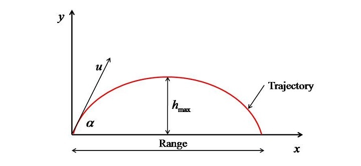
Here, "u" is the velocity with which the projectile is being projected. 𝛼 is the angle of projection of the projectile. The path taken up by the projectile during its flight. Range is the maximum horizontal distance travelled by the projectile. $\mathrm{h_{max}}$ is the maximum height attained by the projectile. Moreover, the time taken up by the projectile to travel the range is called as time of flight.

The projectile motion is studied in three categories −

• Horizontally projected.

• Inclined projected on the level ground.

• Inclined projected but striking at different levels.

In this tutorial we will touch upon all the three cases.

Case 1: Horizontally Projected

In the first case, the projectile is fired from an elevated place with only horizontal velocity (𝑢) and will strike the ground after some distance R as shown in figure given below.

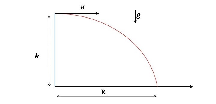
The relation between h, R, and t (time of flight) from the equation of motions can be written as −

$$\mathrm{h=\frac{1}{2}gt^{2}}$$

$$\mathrm{R=ut}$$

To model it in Python, first we have to understand first that what is given and what is required. For that, we will start with a problem.

Example 1

Let suppose a plane at a height of 900 m with a uniform horizontal velocity of 140 m/s releases a packet of food. At what horizontal distance the packet will fall.

In this problem, ℎ and 𝑢 are given and 𝑅 is required. The program will be as follows −

First, take data from the user with the help of input() function and define a variable for acceleration due to gravity. As input from the keyboard is stored as string so type cast it into float by writing float in front of intput().

# Input data
h=float(input("Enter the height of object\n"))
u=float(input("Enter initial velocity in m/s \n"))
# acceleration due to gravity
g=9.81

Evaluate "t" from Equation-1 and "R" from Equation-2.

# Time of flight
t=sqrt(2*h/g)
# Range of projectile
R=u*t

But sqrt() function is not defined in regular Python package, so the math module has to be called at the start of the program.

from math import *

Then print the values of time of flight and range as your answer. Here we have used f-string (format string) to simplify the printing process.

# Output
print(f"Time of flight = {t} s")
print(f"Range = {R} m")

Output

Finally, the program output will look like this −

Enter the height of object
900
Enter initial velocity in m/s
140
Time of flight = 13.545709229571926 s
Range = 1896.3992921400697 m

If one wants, then the output can be roundup to few places of decimal by using round function as follows −

# Output
print(f"Time of flight = {round(t,3)} s")
print(f"Range = {round(R,3)} m")

If one wants to plot the trajectory then the range (𝑅) has to be first divided into array of 𝑥 and the position of projectile at different heights (𝑦) has to be obtained then this data can be plotted to get the balls trajectory. This will explain in the second case.

Case 2: Inclined Projected on the Level Ground

In this case, the projectile is fired from a level ground and reaches the same elevation as shown in the figure given below.

In this case the maximum $\mathrm{h_{max}}$ Range (R), and total time of flight (𝑇) is obtained with the help of the following formulas:

$$\mathrm{h_{max}=\frac{u^{2}\sin^{2}\left ( \alpha \right )}{2g}}$$

$$\mathrm{R=\frac{u^{2}\sin(2\alpha)}{g}}$$

$$\mathrm{T=\frac{2\:u\:\sin\left ( \alpha \right )}{g}}$$

The important point is how to evaluate the trajectory of the profile $\mathrm{y(x)}$. Suppose, at some time "t", the projectile is at point a having coordinate (𝑥,𝑦) as shown in the figure given below.

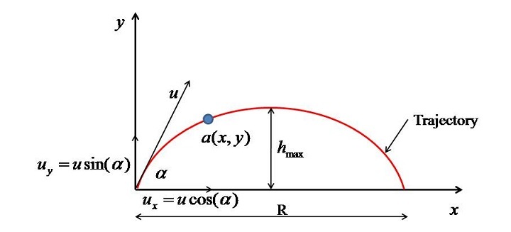
Then the position "y" of the particle as a function of "x" can be obtained by the following derivation.

Equation of motion in "y" direction −

$$\mathrm{y=u_{y}t+\frac{1}{2}a\:t^{2}=u\sin(\alpha )t-\frac{1}{2}gt^{2}}$$

Equation of motion in "x" direction −

$$\mathrm{x=u\cos\left ( \alpha \right )t}$$

$$\mathrm{y=x\tan(\alpha)-\frac{1}{2}\frac{gx^{2}}{u^{2}\cos^{2}\left ( \alpha \right )}}$$

Equation-6 is the one based on which we can easily model the projectile motion and plot the trajectory.

Example 2

As to model it, we will be requiring the arrays so NumPy module will be used moreover, as plotting has to be done, so we will use pylab which is nothing but the matplot.pylab module.

The detailed code and its explanation is shown below −

First numpy and plyab modules are called and imported.

# Importing modules
from numpy import *
from pylab import *

Then u and $\alpha$ are asked from the user. (do not forgot to convert degree into radians with the help of radians() function)

α=float(input("Enter the angle in degrees\n"))
# converting angle in radians
α=radians(α)

# Initial velocity of projectile
u=float(input("Enter initial velocity in m/s \n"))

Then Range and maximum height of projectile with the help of Equations (3) and (4).

# Evaluating Range
R=u**2*sin(2*α)/g


# Evaluating max height
h=u**2*(sin(α))**2/(2*g)

Now array of "x" is created with the help of linspace() function. linspace takes 3 arguments, i.e., the starting point, the ending value, and the number of points to be created between start and stop considering them.

# Creating an array of x with 20 points
x=linspace(0, R, 20)

Then Eq. 6 is solved which will evaluate "y" for different "x".

# Solving for y
y=x*tan(α)-(1/2)*(g*x**2)/(u**2*(cos(α))**2 )

Then plot() function is used to plot the data and some decoration is done to make the plot meaningful. If you want then you can save the figure with the help of savefig() function.

Here we have given the figure number as 1 and to increase the visibility of figure the dpi has been set to 300 by using the function figure().

# Data plotting
figure(1,dpi=300)
plot(x,y,'r-',linewidth=3)
xlabel('x')
ylabel('y')
ylim(0, h+0.05)
savefig('proj.jpg')
show()

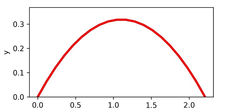
For 𝑢=5 m/s and 𝛼=30∘, the output of the above program will be as follows −

If one wants to print the data in the tabulated form, then the following program snippet can be of great help.

print(f"{'S. No.':^10}{'x':^10}{'y':^10}")
for i in range(len(x)):
   print(f"{i+1:^10}{round(x[i],3):^10}{round(y[i],3):^10}")

Example

The full program code will look like −

# Importing modules
from numpy import *
from pylab import *

α=float(input("Enter the angle in degrees\n"))
# converting angle in radians
α=radians(α)

# Initial velocity of projectile
u=float(input("Enter initial velocity in m/s \n"))

# Evaluating Range
R=u**2*sin(2*α)/g

# Evaluating max height
h=u**2*(sin(α))**2/(2*g)

# Creating array of x with 50 points
x=linspace(0, R, 20)

# Solving for y
y=x*tan(α)-(1/2)*(g*x**2)/(u**2*(cos(α))**2 )
# Data plotting

figure(1,dpi=300)
plot(x,y,'r-',linewidth=3)
xlabel('x')
ylabel('y')
ylim(0, h+0.05)
savefig('proj.jpg')
show()

print(f"{'S. No.':^10}{'x':^10}{'y':^10}")
for i in range(len(x)):
   print(f"{i+1:^10}{round(x[i],3):^10}{round(y[i],3):^10}")

One more thing we can check is what happens when the projectile is fired at different angles and then plot them. This will help you a lot in understanding how to bundle a code into a function.

In Python, a single line function is defined with the help of lambda as −

f= lambda {arguments}: {output statement}

But as you can see that there are many lines of codes so this will not work instead we will be writing it with the help of def which has the body as follows −

def (arguments):
   statements1
   statement 2
   .
   .
   .

Here we will bundle all the statements after the one where we ask u from the user into on function Projectile_Plot. The function accepts two arguments, i.e., u and $\alpha$ as follows −

# Projectile Function
def Projectile_Plot(u,α):

   # for pronging legend
   αd=α
   
   # converting angle in radians
   α=radians(α)
   
   # Evaluating Range
   R=u**2*sin(2*α)/g
   
   # Evaluating max height
   h=u**2*(sin(α))**2/(2*g)
   
   # Creating array of x with 20 points
   x=linspace(0, R, 20)
   
   # Solving for y
   y=x*tan(α)-(1/2)*(g*x**2)/(u**2*(cos(α))**2 )
   
   # Data plotting
   figure(1,dpi=300)
   plot(x,y,'-',linewidth=2,label=f'α = {αd}')
   xlabel('x')
   ylabel('y')
   ylim(0, h+0.05)
   legend()
   savefig('proj2.jpg')

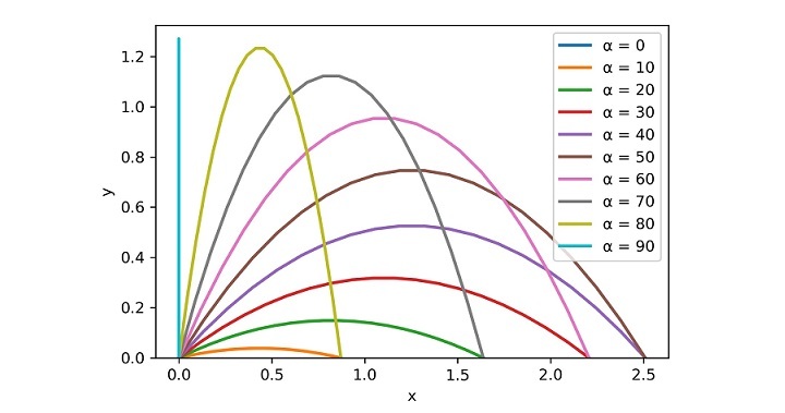
Finally, for a velocity of 5 m/s the projectile motion can be plotted with the help of the following code (Here you should understand that as the angle will be varying so for loop has to be used for it) −

# Input data
# Initial velocity of projectile
u=float(input("Enter initial velocity in m/s \n"))
for i in range(0,100,10):
Projectile_Plot(u,i)
show()

Output

The program output will be as follows −

Case 3: Inclined projected but striking at different levels

In this section, I will show you how to model the projectile when the takeoff and landing points of projectile are not at same elevation as shown in figure given below.

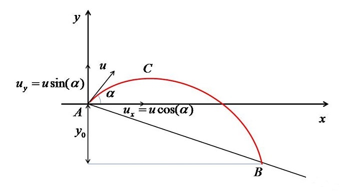
In this case it can be seen that the projection point (A) is $𝑦_{0}$ units higher than the landing point (B).

The method of analysis will be as follows −

Applying equation of motion in vertical direction −

$$\mathrm{s=u_{y}t+\frac{1}{2}a_{y}t^{2}}$$

But $\mathrm{u_{y}=u\sin(\alpha)}$ and $a_{y}=-g$ (i.e. the acceleration due to gravity). so the Eq. 7 then becomes:

$$\mathrm{y=u\sin(\alpha)t-\frac{1}{2}gt^{2}}$$

The time required to reach point B has to be evaluated as follows −

When the projectile reach B then y will get replaced by $−𝑦_{0}$ as this is below the X-axis. Hence, Equation-8 gets converted to −

$$\mathrm{-y_{0}=u\sin(\alpha)t-\frac{1}{2}gt^{2}}$$

For better understanding it can be simplified as −

$$\mathrm{gt^{2}-2u\sin(\alpha)t-2y_{0}=0}$$

Now this quadratic equation (i.e. Eq. 10) has to be solved to get t.

Finally, the horizontal range can be evaluated as −

$$\mathrm{R=u\cos(\alpha)t}$$

In this case, as we have to solve the quadratic equation (i.e. Equation-10), so to simplify the task we will use NumPy (Numerical Python). Before we program this projectile motion let me show you how to find the roots of a quadratic equation using NumPy.

Roots of Equation in NumPy

Let say we want to find the roots of the equation

$$ax^{2}+bx+c=0$$

Then the first step is to call NumPy as follows −

from numpy import *

Then the coefficients of the above polynomial are then stored in a array as follows (Note: starting from the highest to the lowest power of polynomial) −

coeff=array([a,b,c])

Then the function roots() is called to solve the roots as follows −

r1,r2=roots(coeff)

As this is a quadratic equation so we already know that two roots will be there so we are storing them in variables "r1" and "r2". But if the degree of polynomial increases, then the number of roots variables have to be increased accordingly. The examples shown below will clear the procedure shown above.

Finding the roots of polynomial x² - 5x + 6 = 0

# Importing NumPy
from numpy import *

# The polynomial is x^2 -5x+6=0
# The coefficients of the above equation are:
a=1
b=-5
c=6

# Creating array of coefficients
coeff=array([a,b,c])

# Calling function to find the roots
r1,r2=roots(coeff)

# Printing result
print(f"r1 = {round(r1,3)} and r2 = {round(r2,3)}")

On execution, it will produce the following output −

r1 = 3.0 and r2 = 2.0

Finding the roots of polynomial x³- 2x²- 5x + 6 = 0 

# Importing NumPy
from numpy import *

# The polynomial is x^3-2x^2-5x+6=0

# The coefficients of the above equation are:

a=1
b=-2
c=-5
d=6

# Creating array of coefficients
coeff=array([a,b,c,d])

# Calling function to find the roots
r1,r2,r3=roots(coeff)

# Printing result
print(f"r1 = {round(r1,3)}, r2 = {round(r2,3)} and r3 = {round(r3,3)}")

On execution, you will get the following output −

r1 = -2.0, r2 = 3.0 and r3 = 1.0

Now we are in a position to solve for the inclined projectile motion.

Example 3

A bullet is fired at 100 m above the ground with a velocity and angle of 100 m/s and $45^{0},$ respectively. Following things are to be evaluated −

• Flight time

• Range of flight

• Maximum height of projectile

Solution

Import the packages −

from numpy import *
from pylab import *

Supply the input data −

# Velocity at the start
u=100
# Angle of projectile at start
α=radians(45)
# Elevation of starting point above the ground
y0=100
# Acceleration due to gravity
g=9.81

Evaluate the time of flight −

# Time of flight
a=g
b=-2*u*sin(α)
c=-2*y0

# coefficient array
coeff=array([a,b,c])

# finding roots
t1,t2=roots(coeff)
print(f"t1= {t1} and t2= {t2}")

This will return two roots, i.e., two values of time. The non-negative value will be accepted.

The maximum height of the projectile will be obtained by formula −

$$\mathrm{h_{max}=\frac{u^{2}\sin^{2}(\alpha)}{2g}+y_{0}}$$

# From the throwing point
h1=u**2*(sin(α))**2/(2*g)

# total
h_max=h1+y0
print(f"h_max= {round(h_max,3)} m")

Range will be evaluated by Eq. 11 as follows −

R=u*cos(α)*max(t1,t2)
# max(t1,t2) will return the positive value

print(f"R= {round(R,3)} m")

Therefore, the full program and the program output will be as follows −

# Importing packages
from numpy import *
from pylab import *

# Input data
# Velocity at the start
u=100

# Angle of projectile at start
α=radians(45)

# Elevation of starting point above the ground
y0=100

# Acceleration due to gravity
g=9.81

# Time of flight
a=g
b=-2*u*sin(α)
c=-2*y0

# coefficient array
coeff=array([a,b,c])

# finding roots
t1,t2=roots(coeff)
print(f"t1= {t1} and t2= {t2}")

# Maximum Height
# From the throwing point
h1=u**2*(sin(α))**2/(2*g)

# total
h_max=h1+y0
print(f"h_max= {round(h_max,3)} m")

# Range
R=u*cos(α)*max(t1,t2)
#max(t1,t2) will return the positive value

print(f"R= {round(R,3)} m")

When you run the program code, it will produce the following output −

t1= 15.713484026367722 and t2= -1.2974436352046743
h_max= 354.842 m
R= 1111.111 m

Plotting the Projectile Motion

Now the task is to plot this projectile motion. The equation will be the same as what I have used previously, i.e.,

$$\mathrm{y=x\tan(\alpha)-\frac{1}{2}\frac{gx^{2}}{u^{2}\cos^{2}(\alpha)}}$$

Plotting procedure will be −

• First pylab is imported

• Considering (0,0) and $(R,-y_{0})$ the inclined plane is drawn.

• Then array of x is created from 0 to R.

• Eq. 6 is solved to obtain array of y for corresponding x.

• Finally plotting the (𝑥,𝑦) using plot() function.

The complete Python code and plot are as follows −

from pylab import *
# Figure name
figure(1, dpi=300)

# Plotting inclined surface
plot([0,R],[0,-y0],linewidth=5)

# plotting y=0 line
plot([0,R],[0,0],'k',linewidth=1)

# Array of x
x=linspace(0,R,50)

# Evaluating y based on x
y=x*tan(α)-(1/2)*(g*x**2)/(u**2*(cos(α))**2 )

# Plotting projectile
plot(x,y,'r-',linewidth=2)
xlabel('x')
ylabel('y')
savefig("Inc_Proj.jpg")
show()

It will produce the following plot −

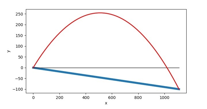
The point to note here is that the projectile can only be drawn once you have evaluated the Range of projectile. Therefore, you will evaluate Range first then will use the code for its plotting.