How To Display Text Labels In The X-axis Of Scatter Chart In Excel?

A strong visualisation method for showing the relationship between two variables is a scatter chart. Excel plots numerical values on the X and Y axes by default. The X?axis can occasionally be labelled with text rather of numbers, though.

In this article, we'll look at a step?by?step method for carrying out this task in Excel. The capability to display text labels on the X?axis can result in a clearer and more useful visualisation, regardless of whether you want to build a scatter chart for business, study, or personal use. We'll assume you have a fundamental understanding of Excel and its features throughout this course. Let's get started and discover how to display text labels in the X?axis of a scatter chart in Excel now, shall we?

Display Text Labels In The X?axis Of Scatter Chart

Here we will format the chart to complete the task. So let us see a simple process to know how you can display text labels on the X?axis of a scatter chart in Excel.

Step 1

Consider an Excel sheet where you have a scatter chart similar to the below image.

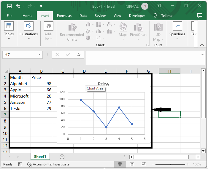
First, right?click on the chart line and select Format Data Series.

Right click > Format data series.

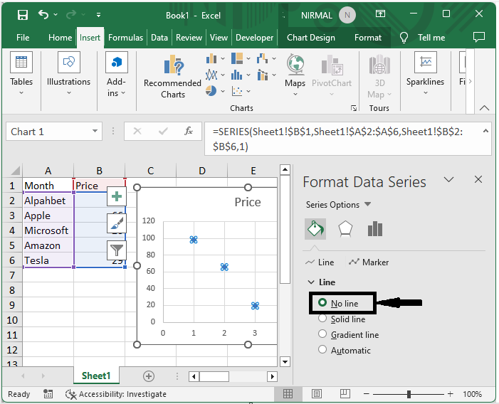
Step 2

Then click on fill, select no fill, and close the format menu to complete the task.

Fill > No fill > Close.

Then you can see that the text labels are on the x axis of the scatter chart.

This is how you can display text labels on the x axis of a scatter chart in Excel.

Conclusion

In this tutorial, we have used a simple example to demonstrate how you can display text labels on the X?axis of a scatter chart in Excel to highlight a particular set of data.