
Article Categories
- All Categories
-
 Data Structure
-
 Networking
-
 RDBMS
RDBMS
-
 Operating System
-
 Java
Java
-
 MS Excel
-
 iOS
iOS
-
 HTML
HTML
-
 CSS
CSS
-
 Android
-
 Python
-
 C Programming
-
 C++
C++
-
 C#
C#
-
 MongoDB
-
 MySQL
MySQL
-
 Javascript
-
 PHP
PHP
-
 Economics & Finance
How to Copy and Paste Only Non-Blank Cells in Excel?
Generally, in Excel, a list may or may not contain empty cells, and when we want to copy the cells with only values, then we can use the method mentioned in this tutorial. If we try to copy and paste in the default way, then empty cells will also be copied by default. If we try to do this manually, it can be time-consuming. Read this tutorial to learn how to copy and paste only non-blank cells in Excel.
Copy and Paste Only Non-Blank Cells Using VBA
Here first we will open the VBA application, then insert a module, copy the code into it, and finally run the code to complete our task. Let us see a simple process to know how we can copy and paste only non-blank cells using the VBA application.
Step 1
Consider an Excel sheet with data similar to the image below. Now right-click on the sheet name and select view code to open the VBA application, then click on insert in the VBA application and click module.
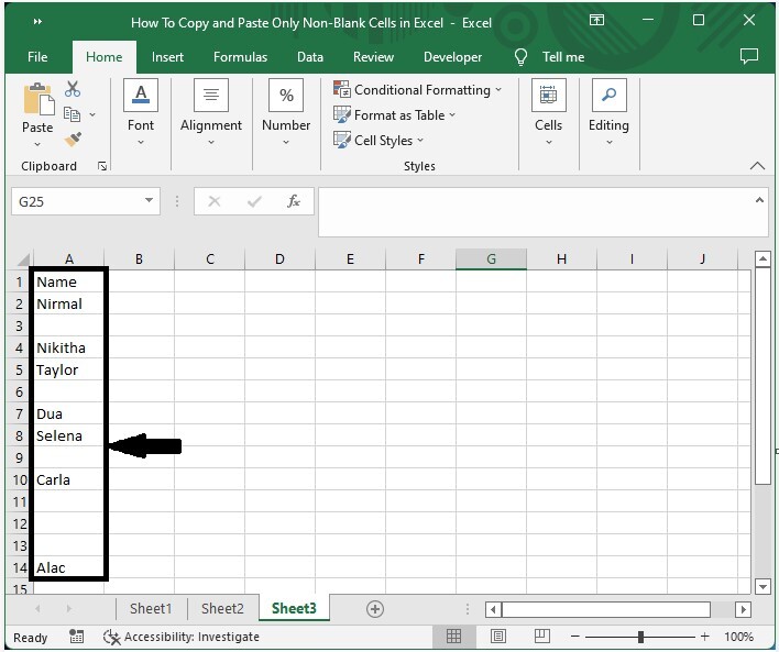
Right click > view code > insert > module
Step 2
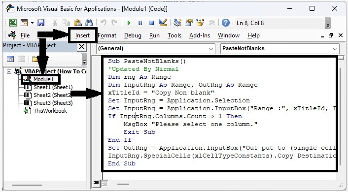
Type the following program code in the textbox, as shown in the image below.
Program
Sub PasteNotBlanks()
'Updated By Nirmal
Dim rng As Range
Dim InputRng As Range, OutRng As Range
xTitleId = "Copy Non blank"
Set InputRng = Application.Selection
Set InputRng = Application.InputBox("Range :", xTitleId, InputRng.Address, Type:=8)
If InputRng.Columns.Count > 1 Then
    MsgBox "Please select one column."
    Exit Sub
End If
Set OutRng = Application.InputBox("Out put to (single cell):", xTitleId, Type:=8)
InputRng.SpecialCells(xlCellTypeConstants).Copy Destination:=OutRng.Range("A1")
End Sub
Step 3
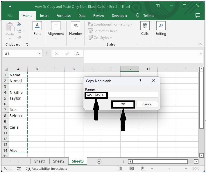
Then save the sheet as a macro-enabled workbook, click on F5, select the range of our cells that you want to copy, and click OK.
Save > F5 > Range > OK
Step 4
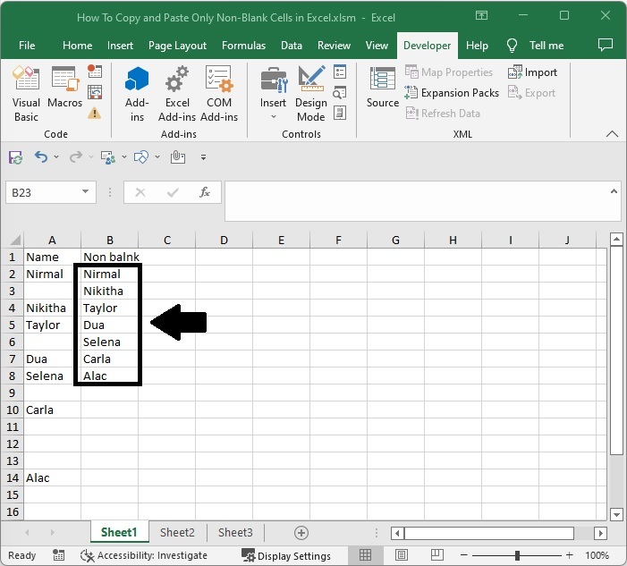
Then select the cells where you want to create the output from and click OK.
Output cell > OK
Conclusion
In this tutorial, we used a simple example to demonstrate how we can copy and paste only non-blank cells in Excel.

1K+ Views
