How to check if one list against another in Excel?

There are cases when we need to compare multiple sheets for consolidating the data in a single sheet against similar entries. Manually this task may need huge manpower as well as time. On the other side the same data can be consolidated by using a one or two formulas and copying the same in all respective sheets. In this article, we will be working on the following formulas for identifying one list against another.

• =VLOOKUP(lookup_value, table_array, column_index_number, [range_lookup])

• =MATCH(lookup_value, lookup_array, [match_type])

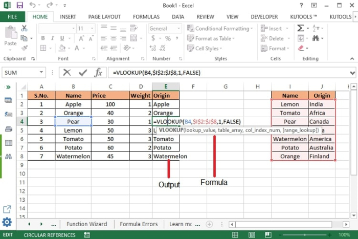
Check one list against another using VLOOKUP function

Step 1 − We have taken the sample data as shown below.

Step 2 − Now enter the below formula in a separate column where you want to get the matching values of another column against the first column.

=VLOOKUP(lookup_value,table_array,column index number,False (for similar values) or TRUE (for exact match))

Sample formula for below dataset − =VLOOKUP(B2,$I$2:$J$8,1,FALSE)

Points to be noted

• In the formula, B2 is the first cell of the list you want to check if against to another one, I2:J7 is the second list you want to check based on.

• This formula can also be used to check one list against another

=IF(COUNTIF($I$2:$I$7,B2)>0,TRUE,FALSE)

Formula Syntax Description

Argument

Description

=VLOOKUP(lookup_value, table_array, column_index_number, [range_lookup])

V lookup is used when we need to compare two rows of a single sheet of different sheets. Lookup_value specifies the cell address whose value to be looked up in the selected array. Table_array specifies the array of data in which the selected cell value to be looked up. Column index number specifies the column number of selected table array whose value to be returned against each lookup value. Range lookup value may have two options False or True. If false then function will return similar values. If true, the function will return exact matches only.

Check one list against another using MATCH function

The MATCH function returns the cell address where the value of selected cell is available instead of the exact value. In the same data which we have used in the above function, paste the following formula in a new column.

=MATCH(lookup_value, lookup_array, [match_type])

Sample formula =MATCH(B2,$I$2:$I$8,0)

The output will be as shown below −

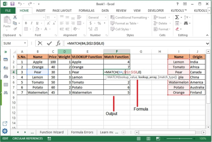
Here is the final output of both the functions −

Formula Syntax Description

Argument

Description

MATCH(lookup_value, lookup_array, [match_type])

The MATCH function searches for a specified item in a range of cells, and then returns the relative position of that item in the range. Lookup_value specifies the cell address whose value to be looked up in the selected array. Lookup_array specifies the array of data in which the selected cell value to be looked up. Match_type here you can enter 1 for less than value, 0 for exact match, -1 for greater value.

Conclusion

Finally, these two functions are widely used for comparing the data of columns within a single dataset or different sheets. Along with these, many other combinational functions can also be used for this purpose. The same will be explained in upcoming articles. Keep learning and keep exploring.