
Article Categories
- All Categories
-
 Data Structure
-
 Networking
-
 RDBMS
RDBMS
-
 Operating System
-
 Java
Java
-
 MS Excel
-
 iOS
iOS
-
 HTML
HTML
-
 CSS
CSS
-
 Android
-
 Python
-
 C Programming
-
 C++
C++
-
 C#
C#
-
 MongoDB
-
 MySQL
MySQL
-
 Javascript
-
 PHP
PHP
-
 Economics & Finance
How to calculate running total /average in Excel?
The climax of a continuing sequence of partial totals of a particular data collection is what is known as a cumulative total, which is also referred to as a running total in certain circles. The use of a "running total," which shows the total as it increases and allows for the accumulation of data to be summarised as it occurs over time, is required in order to present the summary of the data.
This widely common method is used on a day-to-day basis by students and professionals who are assigned the task of using Excel to compute and calculate a range of intricate data and calculations.
It is not necessary to spend the time recording the sequence itself if you have a running total to keep track of the progress since it is not vital to know the particular numbers that are being used in the sequence.
Step 1
Although this calculation can seem to be very complicated at first glance, the idea behind it is really quite simple and one that many of us are exposed to on a daily basis, regardless of whether or not we are the ones actually using it.
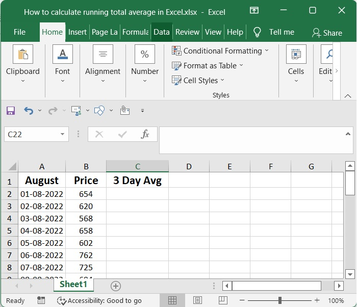
All of August's daily data can be found in the A column, while prices can be found in the B column. We need the average of the last three days in the C column.
Step 2
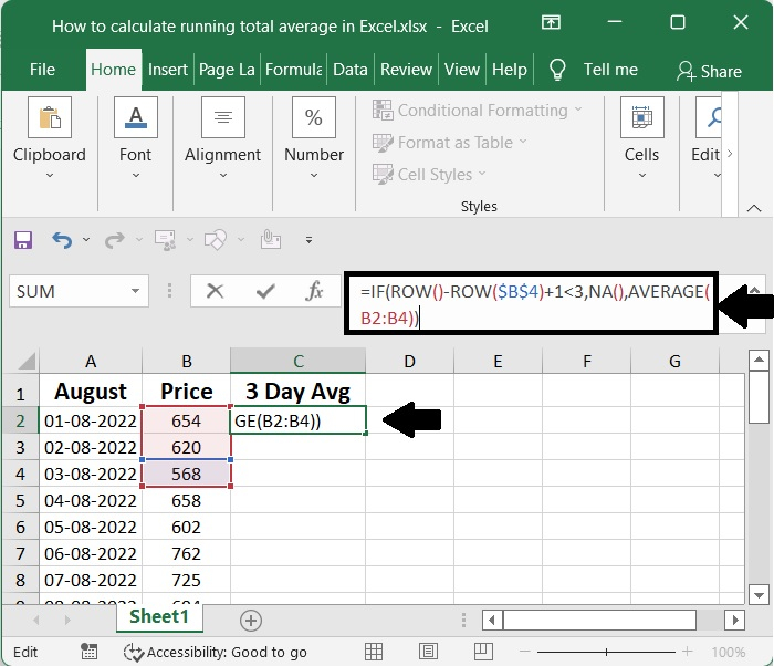
Checking the current row number and exiting with the #NA code when there are less than n values is one approach to make it very evident that there is insufficient data. For the average for the last three days, you may, for instance, use
=IF(ROW()-ROW($B$4)+1<3,NA(),AVERAGE(B2:B4))
The first component of the formula consists of nothing more than the generation of a "normalized" row number, which begins with 1.
Step 3
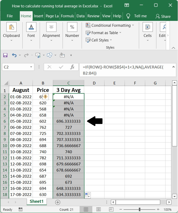
Depending on the layout of the worksheet and whether or not it's critical that all averages be computed using the same amount of data points, there are a few different approaches to take.
Because the AVERAGE function is set to automatically disregard text values and cells that are empty, it will continue to compute an average even if there are less values. The reason why it "works" in both C2 and C5 is because of this.
Step 4
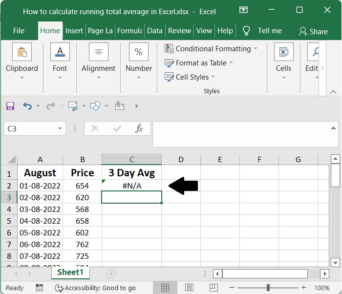
#N/A is what the algorithm gives back if the current row number is lower than 3. In every other case, the algorithm will produce a moving average just as it did previously. This replicates the behaviour of the Moving Average function included in the Analysis Toolpak, which generates the value #N/A until the first full period has been achieved.
Conclusion
In this tutorial, we used a simple example to demonstrate how you can calculate the running average in Excel.

593 Views
