How to border every 5/n rows in Excel?

In Excel, the lines that make it up a cell’s border are referred to as boxes by maintain borders, we are able to frame any data and give it a defined boundary in an appropriate manner. You can highlight specific values by outlining summarized values or separating data into ranges of cells, additionally, you can place borders around individual cells.

Adding borders is one of the greatest and easiest ways to make a spreadsheet seem attractive, and this is especially true if the spreadsheet is going to be printed. However, if you are consistent including new data in your spreadsheet, then you will also need to consistently update the borders of the spreadsheet.

Have you ever wished to select every 5/n row in Excel and then format them in a specified range? If so, you can do so with this function. In point of fact, there are a variety of solutions to choose from for this issue. In this article, I will discuss three different approaches for applying a border to every 5/n rows within a given range in Excel.

Border Every 5/n Rows With Filter Command in Excel

In Excel, we can make use of an additional help column to identify each 5/n row, after which we can filter these rows in Excel and give them boundary lines. Let’s understand it step by step with an example.

Step 1

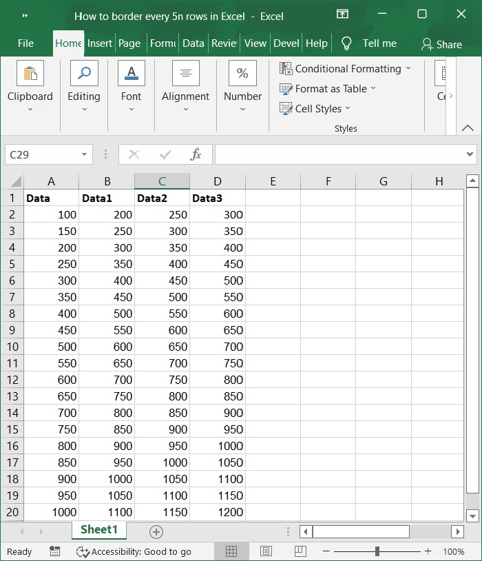
In our example, we must create sample data. As shown in the below screenshot.

Step 2

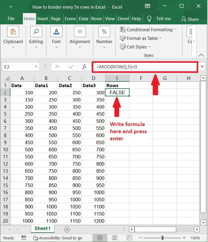
After typing Rows into the first cell of an empty column that is adjacent to the original range, enter the formula into the second cell. Refer to the below screenshot.

Formula

=MOD(ROW(),5)=0

Step 3

After that, drag the Fill Handle to the range where you want this formula to be applied and let go of it. Checkout the below screenshot.

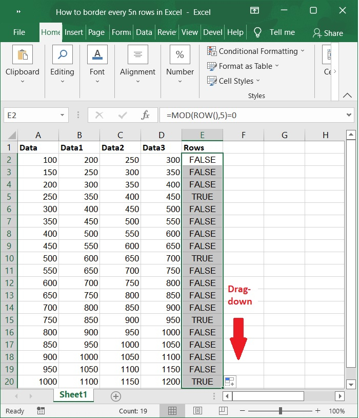
Important Note − The number 5 in the formula =MOD(ROW(),5)=0 indicates every 5th row; however, this value can be altered to suit your requirements.

Step 4

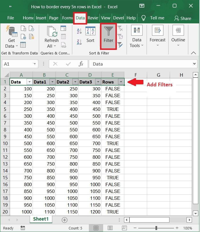
After selecting the Rows column, go to the Data menu and then click on Filter. Refer to the below screenshot.

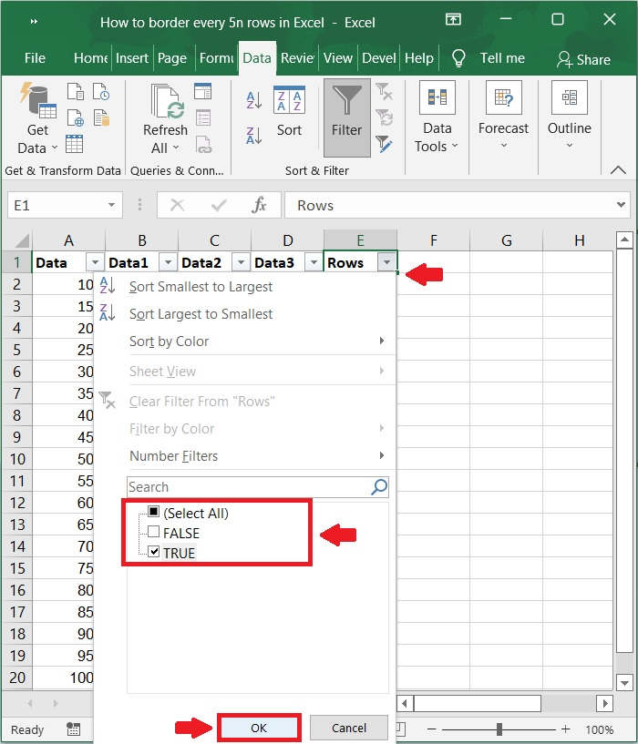
Step 5

Click the arrow in the first cell of the Rows column, then un-select all of the options with the exception of the TURE option, and then click the OK button when you are finished. Please refer to the screenshot below for the same.

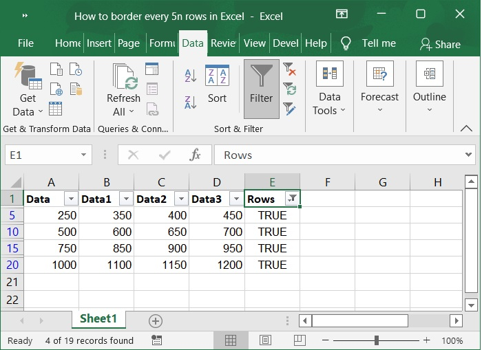
Step 6

Now, you can see the filtered-out row’s columns. See the below screenshot for the same.

Step 7

After making sure that the heading row is not selected, click the arrow next to the Border button on the Home tab, and then select All Borders from the drop-down menu that appears. Refer to the below screenshot for the same.

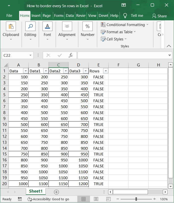
Step 8

Click the arrow in the first cell of the Rows column, then select all of the options and then click the OK button when you are finished. You will also see that all of the borders are added to every 5th row simultaneously. Please refer to the below screenshot.

Conclusion

In this tutorial, we used a simple example to demonstrate how you can add border every 5th row using the filter command in Excel.