
Article Categories
- All Categories
-
 Data Structure
-
 Networking
-
 RDBMS
RDBMS
-
 Operating System
-
 Java
Java
-
 MS Excel
-
 iOS
iOS
-
 HTML
HTML
-
 CSS
CSS
-
 Android
-
 Python
-
 C Programming
-
 C++
C++
-
 C#
C#
-
 MongoDB
-
 MySQL
MySQL
-
 Javascript
-
 PHP
PHP
-
 Economics & Finance
How to Apply Conditional Formatting Search for Multiple Words in Excel?
Assume we have a list of texts where each cell contains multiple words and another list that contains words from the other list, and you want to highlight the cells where these words are present so we can use conditional formatting searches for multiple words to solve the problem in Excel. This tutorial will help you understand how you can apply conditional formatting to a search for multiple words in Excel.
Applying Conditional Formatting Search for Multiple Words in Excel
Here, we will first name a list and then use the name in the formatting formula. Let us see a simple process to apply conditional formatting to multiple word searches in Excel. In the below example, we will highlight the words that contain words from another list.
Step 1
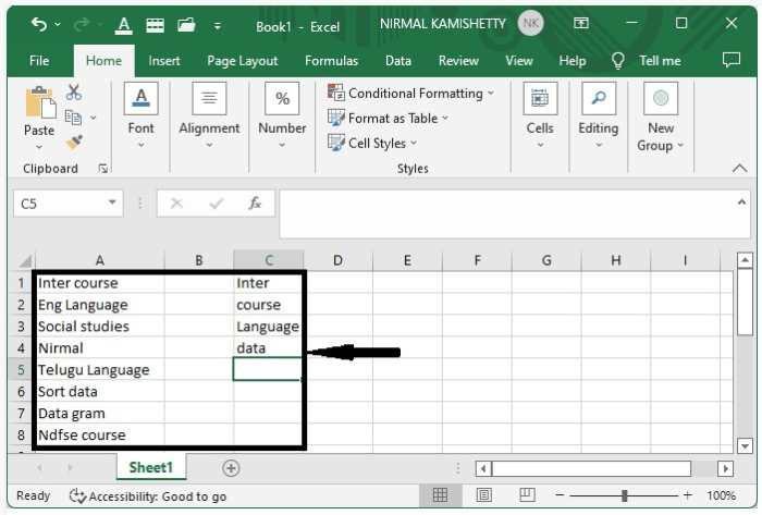
Assume we have an excel sheet with data similar to the data shown in the screenshot below. The cells in row A contain a list of multiple words, while the cells in row C contain single words from the list of cells in row A.
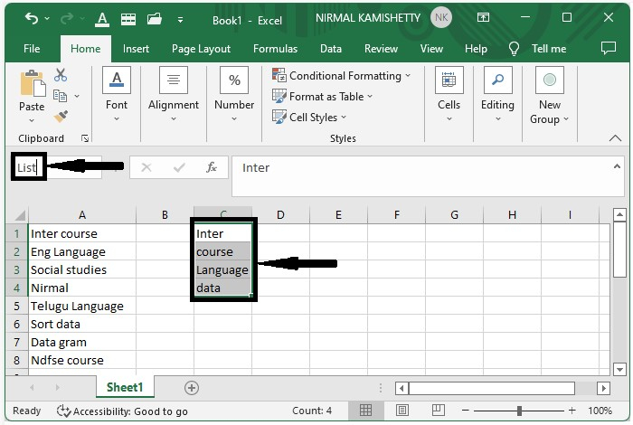
Now select the words and name them as a list, as shown in the below image.
Step 2
Now select the data, click on conditional formatting, and select a new rule under the home of the Excel ribbon. A new popup will be opened.
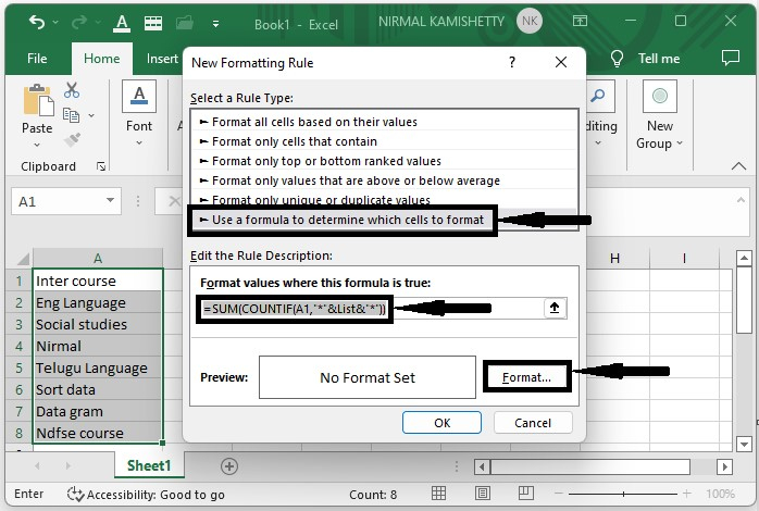
Then select use the formula, enter the formula as =SUM(COUNTIF(A1,"*"&List&"*")) in the formula box, and click on format as shown in the below image.
Step 3
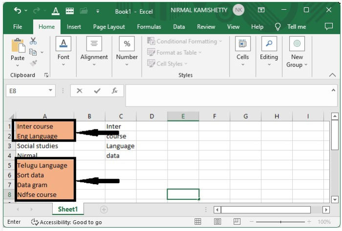
After clicking on format, in the new popup, select the colour in the fill and click on OK, and again click on OK to successfully highlight the data. Our final result will look similar to the below image.
Conclusion
In this tutorial, we used a simple example to demonstrate how you can apply conditional formatting to a search for multiple words in Excel to highlight a particular set of data.

10K+ Views
