
Article Categories
- All Categories
-
 Data Structure
-
 Networking
-
 RDBMS
RDBMS
-
 Operating System
-
 Java
Java
-
 MS Excel
-
 iOS
iOS
-
 HTML
HTML
-
 CSS
CSS
-
 Android
-
 Python
-
 C Programming
-
 C++
C++
-
 C#
C#
-
 MongoDB
-
 MySQL
MySQL
-
 Javascript
-
 PHP
PHP
-
 Economics & Finance
How to Apply Colour Gradient Across Multiple Cells in Excel?
You could have added different colours to cells in Excel, but have you tried adding different shades of the same colour to the cells? It is possible to add shades of the same colour to the spreadsheet cells. Adding shades of the same colour will look better than using different colours. This tutorial will help you understand how you can add a colour gradient across multiple cells in Excel by following some simple steps.
Applying Colour Gradient Across Multiple Cells in Excel
Here, we will first apply the conditional formatting to cells and select gradient colours. Let us see a simple process to apply a colour gradient across multiple cells in Excel.
Step 1
Let us consider that we have an Excel sheet that contains data similar to the data shown in the below screenshot.
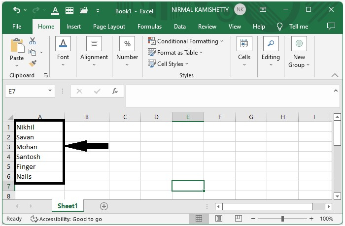
Now select the cells where you want to apply a colour gradient and right-click, then select format cells. A new pop-up window will be opened, similar to the below image.
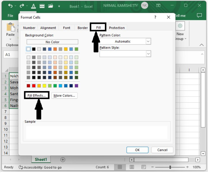
Now, in the new pop-up window, click on the fill effect once more, as shown in the above image; a new pop-up window will be opened.
Step 2
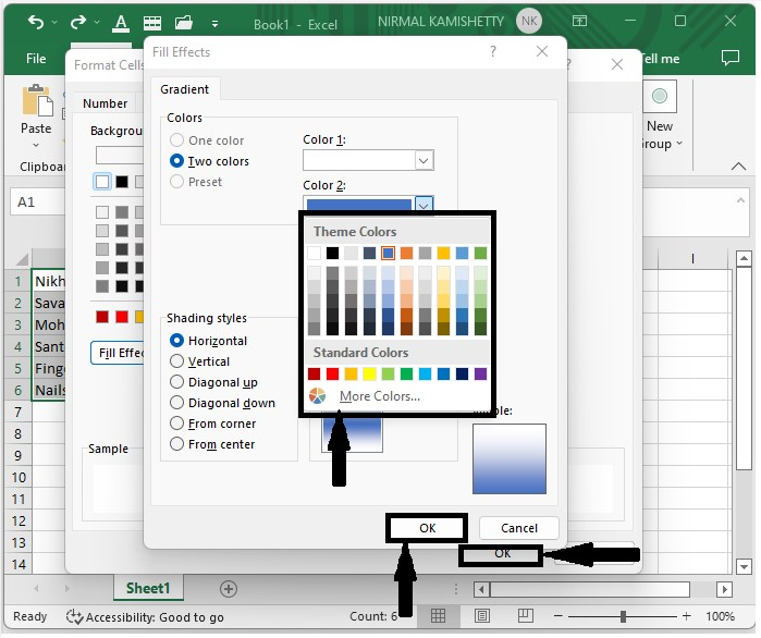
In the new pop-up, select the colour you want to use to fill in the cells, then select the horizontal shading style. Click OK to close the pop-up, then OK again on the previous pop-up to close the pop-up, as shown in the below image.
Our final output will be very similar to the below screenshot.
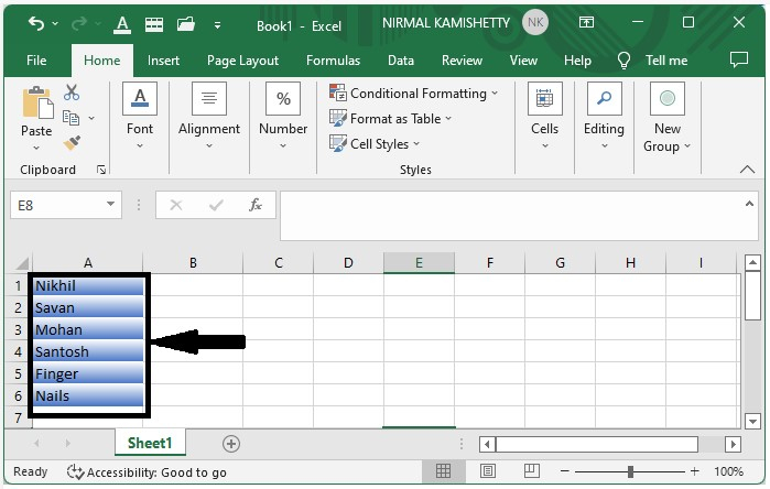
As we can see, we have successfully added the colour gradient to the cells.
Conclusion
In this tutorial, we used a simple example to demonstrate how you can apply a colour gradient across multiple cells in Excel to highlight a particular set of data.

3K+ Views
