
 Data Structure
 Networking
 RDBMS
RDBMS Operating System
 Java
Java MS Excel
 iOS
iOS HTML
HTML CSS
CSS Android
 Python
 C Programming
 C++
C++ C#
C# MongoDB
 MySQL
MySQL Javascript
 PHP
PHP
- Selected Reading
- UPSC IAS Exams Notes
- Developer's Best Practices
- Questions and Answers
- Effective Resume Writing
- HR Interview Questions
- Computer Glossary
- Who is Who
Excel tips for the power users
Excel is one of the most commonly used business software on the market. And yet not everyone is able to fully utilize it. By using these tips you can create impressive spreadsheets that communicate effectively and make your point clearly and quickly.
VLOOKUP
It helps you search data that’s scattered across different sheets and workbooks and bring those sheets into a central location to create reports and summaries. It helps you find information in large data tables such as inventory lists. To insert this, select the Formulas tab, and then click on Insert Function. A box appears that allows us to select any of the functions available in Excel. The system would return us a list of all lookup-related functions in Excel. Enter the cell that contains your reference number, then enter the range of cells in the sheet or workbook from which you need to pull data, the column number for the data point you’re looking
for, and either “True” (if you want the closest reference match) or “False” (if you require an exact match).
IF Formulas
IF and IFERROR are the two most useful IF formulas in Excel. IF formulas lets you pull in just the data you need. IFERROR is a variant of the IF Formula. It lets you return a certain value (or a blank value) if the formula you’re trying to use returns an error. If you’re doing a VLOOKUP to another sheet or table, for example, the IFERROR formula can render the field blank if the reference is not found.
PivotTables and Pivot Chart
PivotTables are essentially summary tables that let you count, average, sum, and perform other calculations according to the reference points you enter. PivotChart lets you quickly and easily look at complex data sets in an easy-to-digest way. You can preview a chart by hovering your mouse over that option. To create PivotTable and pivot chart, first ensure your data is titled appropriately, then select the pivot chart or pivot table icon on the Insert tab.
Flash Fill
This feature solves one of the most frustrating problems of Excel by pulling needed pieces of information from a concatenated cell. IT has ability to take a part of the data entered into one column of a worksheet table and enter just that data in a new table column using only a few keystrokes. Flash Fill can automatically add data, formatted the way you want without using formulas.
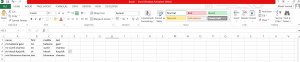
Rather than manually entering first, middle, or last names in respective columns (or attempting to copy an entire client name from column A and then editing out the parts not needed in the First Name, Middle Name, and Last Name columns), you can use Flash Fill to quickly and effectively do the job.
Click Home > Fill > Flash Fill, and Excel will automagically extract the first name from the remaining people in your table.
Conditional Formatting
Excel spreadsheet is to show large amounts of data in numeric form. This feature lets you easily highlight data points of interest. If you just want to identify cells that contain unusual results, use the Highlight Cells Rules option and define formatting based on a formula or an absolute number.
Select Home tab in the taskbar and choose the range of cells you want to format, then click the Conditional Formatting dropdown. The features you’ll use most often are in the Highlight Cells Rules submenu.
Filter the Contents of a List
For long lists, it’s often helpful to be able to filter the list’s contents. For that task, the built-in filtering option which can easily track data in lists. The data can be numeric, text and dates as well.
To start, you need a list that has headers with no empty rows. Click anywhere within the list and then, on the Data tab, click the Filter button. That displays a small arrow alongside each column header, which you can click to reveal the filter list. Clear any checkbox to filter out cells that match that value. If you’ve chosen the filter list for a column containing dates, you can select by year, month, day or operators like between, before, and after.
Transposing Columns into Rows (and Vice Versa)
Just copy the row or column you’d like to transpose, right click on the destination cell and select Paste Special. A checkbox on the bottom of the resulting popup window is labelled Transpose. Check the box and click OK. Excel will do the rest.
Power View
It is an interactive data exploration and visualization tool that can pull and analyse large quantities of data from external data files.
Go to Insert > Reports. It creates interactive, presentation-ready reports. Reports created with Power View are presentation-ready with reading and full-screen presentation modes. You can even export an interactive version into PowerPoint.
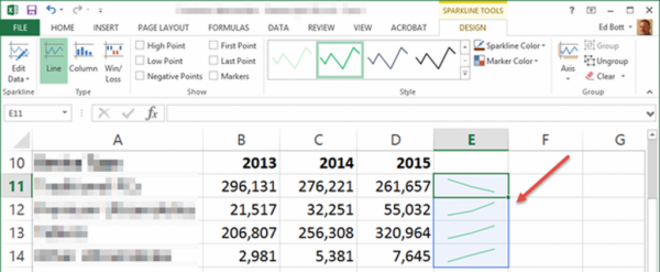
Add Sparklines to Show Visual Trends
They offer a really easy way to help visualize trends in data over time, especially when those trends aren’t immediately obvious from the raw numbers. To insert a Sparkline −
Select an empty cell or group of empty cells in which you want to insert one or more sparklines.
On the Insert tab, in the Sparklines group, click the type of Sparkline that you want to create: Line, Column, or Win/Loss.
In the data box, type the range of the cells that contain the data on which you want to base the sparklines.
The figure below shows a very simplified use of the Line option, which makes it immediately obvious that one of these four rows of data is on a different trend line than the other three.
Quick Analysis
This tool minimizes the time needed to create charts based on simple data sets. Once you have your data selected, an icon appears in the bottom right hand corner that, when clicked, brings up the Quick Analysis menu. Quick Analysis speeds the process of working with simple data sets.
This menu provides tools like Formatting, Charts, Totals, Tables, and Sparklines. Hovering your mouse over each one generates a live preview.
Essential Keyboard Shortcuts
Keyboard shortcuts are the best way to navigate cells or enter formulas more quickly. Some of the common are –
Control-Down/Up Arrow = Moves to the top or bottom cell of the current column
Control-Left/Right Arrow = Moves to the cell furthest left or right in the current row
Control-Shift-Down/Up Arrow = Selects all the cells above or below the current cell
Shift-F11 = Creates a new blank worksheet within your workbook
F2 = opens the cell for editing in the formula bar
Control-Home = Navigates to cell A1
Control-End = Navigates to the last cell that contains data
Alt = Autosums the cells above the current cell
Hopefully these tips and shortcuts Save Time and effort and boost your productivity and proficiency.

283 Views
