
 Data Structure
 Networking
 RDBMS
RDBMS Operating System
 Java
Java MS Excel
 iOS
iOS HTML
HTML CSS
CSS Android
 Python
 C Programming
 C++
C++ C#
C# MongoDB
 MySQL
MySQL Javascript
 PHP
PHP
- Selected Reading
- UPSC IAS Exams Notes
- Developer's Best Practices
- Questions and Answers
- Effective Resume Writing
- HR Interview Questions
- Computer Glossary
- Who is Who
Curve Fitting Models in Software Engineering
Curve fitting is the process of constructing a curve, or mathematical function, that best fits a set of data points, subject to constraints. Curve fitting can include either interpolation, which requires a precise fit to the data, or smoothing, which involves creating a "smooth" function that approximates fits the data.
Regression analysis is a similar topic that focuses on statistical inference problems such as how much uncertainty is present in a curve that is fit to data seen with random errors.
Fitted curves can be used to help in data visualization, predict function values when no data is provided, and describe the connections between two or more variables. Extrapolation is the use of a fitted curve outside the range of the observed data, and it is prone to misinterpretation since it may represent the method used to construct the curve as much as the actual data.
The curve fitting group models investigate the link between software complexity and the number of defects in a program, the number of modifications, or the failure rate using statistical regression analysis. This class of models uses linear regression, nonlinear regression, or time series analysis to determine a connection between input and output variables. The amount of mistakes in a program, for example, is one of the dependent variables. The independent variables are the number of modules modified during the maintenance period, the duration between failures, the expertise of the programmers, the size of the software, and so on.
This category includes the following models −
- error estimation,
- complexity estimation, and
- failure rate estimation.
These are discussed below.
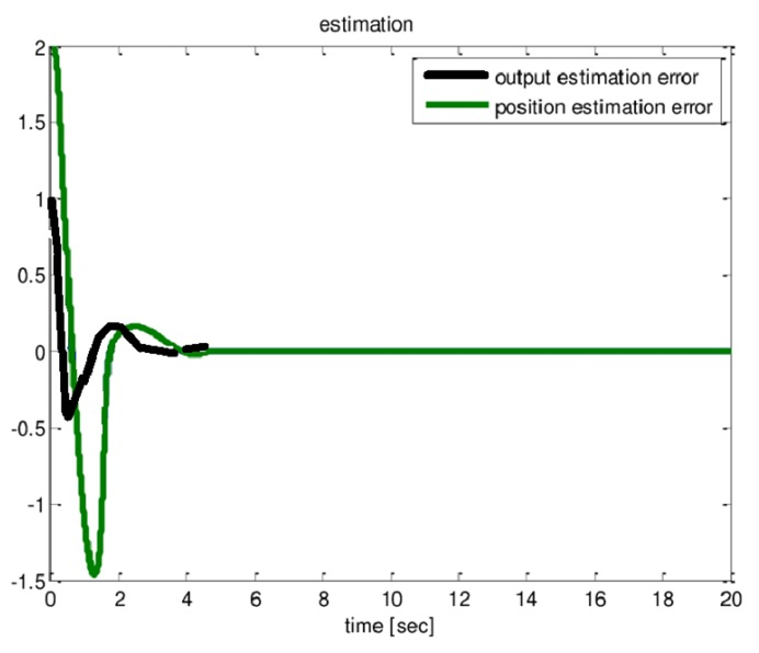
The following graph compares actual to estimated values.
- Error Estimation Model
A linear or nonlinear regression model may be used to estimate the number of mistakes in a program. The following is a basic nonlinear regression model for estimating the total number of initial mistakes in the program, N −
$$\mathrm{N = ∑a_{i}x_{i}+∑b_{i}{x^{2}_{i}}+ ∑x{x^{3}_{i}} + ε}$$
Where,
- xi is the ith error factor,
- ai, bi,are ci model coefficients, and
- ε is an error term.
Software complexity metrics and environmental variables are examples of typical error causes. The majority of curve fitting models have only one error component.
- Complexity Model Estimation
Using the time series method, this model is used to estimate the software complexity, CR. The following is a summary of the software complexity model −
$$\mathrm{CR = a_{0} + {a_{1}}^R + {a_{2}}^{ER} + {a_{3}}^{MR} + {a_{4}}^{IR} + {a_{5}}^{D} + ε}$$
where
- R denotes the release sequence number.
- ER = environmental factor(s) at the time of release R
- MR denotes the number of modules at release R.
- IR is an abbreviation for inter-release interval R.
- D = the number of days between the occurrence of the first error and the occurrence of the second error.
- ε = Error
This model is utilized when the program is assessed throughout time, which implies when new versions of the model are published.
- Failure Rate Model Estimation
This approach is used to estimate software failure rates. Given t1, t2,..., tn failure intervals, an approximate estimate of the failure rate at the ith failure interval is,
$$\mathrm{λ_{i} =\frac{1}{t(i - 1) - t_{i}}}$$
Assuming that the failure rate is monotonically non-increasing, the least squared approach may be used to generate an estimate of this function lambda, i = 1, 2,..., n.
Various Kinds of Curve Fitting
Lines and polynomial curves are used to fit data points. Begin with a first-degree polynomial equation −
$$\mathrm{y = ax + b}$$
This is a sloped line. We already know that a line can link any two locations. A first degree polynomial equation is thus a perfect match between any two locations.
When the order of the equation is increased to a second degree polynomial, we get −
$$\mathrm{y = {a_{x}}^{2} + bx + c}$$
This will fit a basic curve to three points precisely.
When the order of the equation is increased to a third degree polynomial, we get −
$$\mathrm{y = {a_{x}}^3 + {b_{x}}^2 + cx + d}$$
This will fit four spots precisely.
A broader statement would be that it would precisely fit four restrictions. Each restriction can take the form of a point, an angle, or a curve (which is the reciprocal of the radius of an osculating circle). Angle and curvature limitations are most commonly added to the endpoints of a curve and are referred to as end conditions in such situations.
To provide a seamless transition between polynomial curves included inside a single spline, identical termination conditions are typically employed. Higher-order restrictions, such as "the rate of curvature change," might also be imposed. This, for example, would be important in highway cloverleaf design to understand the pressures exerted to an automobile as it follows the cloverleaf and, as a result, to determine appropriate speed limits.
Provided this, the first degree polynomial equation may be a perfect match for a single point and an angle, whereas the third degree polynomial equation may be a perfect fit for 2 points, an angle constraint, and a curvature constraint. Many more added constraint combinations are possible for these and higher order polynomial equations.
Fitting other curves to data points
Other types of curves, such as conic sections (circular, elliptical, parabolic, and hyperbolic arcs) or trigonometric functions (such as sine and cosine), might be utilized in particular situations. When air resistance is disregarded, trajectories of objects under the effect of gravity, for example, follow a parabolic route. As a result, matching trajectory data points to a parabolic curve makes sense. Tides observe sinusoidal patterns, thus tidal data points should be matched to a sine wave, or the sum of two sine waves of different periods if the Moon and Sun effects are also taken into consideration.
Algebraic fit versus geometric fit for curves
In algebraic data analysis, "fitting" typically refers to attempting to identify the curve that minimizes a point's vertical (i.e. y-axis) displacement from the curve (e.g. ordinary least squares). Geometric fitting, on the other hand, attempts to give the greatest visual fit for graphical and picture applications, which generally involves attempting to minimize the orthogonal distance to the curve (e.g. total least squares), or to alternatively incorporate both axes of displacement of a point from the curve. Geometric fits are uncommon since they typically need non-linear and/or repeated calculations, despite the fact that they produce a more aesthetically pleasing and geometrically precise outcome.
Fitting a circle by geometric fit
Coope takes on the challenge of determining the best visual fit of a circle to a set of 2D data points. The approach neatly turns a normally non-linear issue into a linear problem that can be solved without the use of iterative numerical methods, and is thus orders of magnitude quicker than prior strategies.
Fitting an ellipse by geometric fit
The preceding methodology is extended to generic ellipses[2] by including a non-linear step, resulting in a method that is quick while also finding visually appealing ellipses of variable orientation and displacement.
Application to surfaces
While this explanation has focused on 2D curves, most of the reasoning also applies to 3D surfaces, with each patch described by a net of curves in two parametric directions, commonly referred to as u and v. In each direction, a surface can be made up of one or more surface patches.

959 Views
