Batch rename multiple hyperlinks at once in Excel

Excel provides a wide variety of options for generating a hyperlink. If you want to create a link to a certain website, all you have to do is write the URL of the page into a cell, press Enter, and Microsoft Excel will immediately transform your entry into a hyperlink that can be clicked on.

You can use the Hyperlink context menu or the Ctrl + K shortcut to link to another worksheet in an Excel file, or you can link to a specific location in another Excel file. Utilizing a Hyperlink formula, which makes it simpler to generate, copy, and update hyperlinks in Excel, is the quickest method available if you plan to enter a large number of connections that are the same or very similar to one another.

Let’s go step by step and understand how it works.

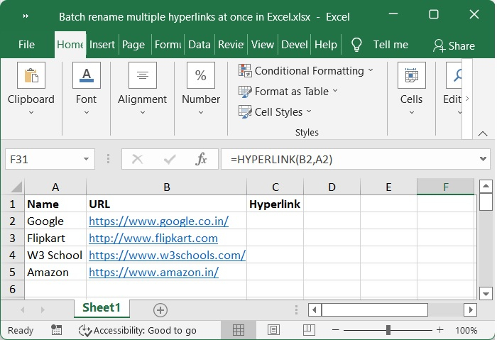
Step 1

Create a sample data which has some website address as shown in the below screenshot.

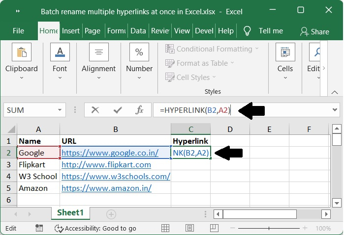
Step 2

Now, select cell C2 and write the formula using the following syntax.

HYPERLINK(link_location, [friendly_name]) 

Let's understand the role of the attributes used in this formula.

Link_location (required) − It is the address of the website or file that is going to be opened. It is possible to supply Link location as either a reference to a cell that contains the link or as a text string encased in quotation marks that contains a path to a file that is stored on a local drive, UNC path that is stored on a server, or URL that is stored on the Internet or intranet. Both of these options are valid. When you click on a cell that has a Hyperlink formula, an error will be generated if the supplied link path does not exist or is broken.

Friendly_name (optional)− It is the text that will be displayed in a cell that serves as a link (also known as jump text or anchor text). If you do not include it, link location will be shown as the link text.

You have the option of providing Friendly name as a numeric value, a text string encased in quotation marks, a name, or a reference to a column in your spreadsheet that includes the link text.

When you select a cell that has a Hyperlink formula, clicking that cell will open the file or web page that was given in the link location parameter.

The following is a representation of the most basic form of an Excel Hyperlink formula, in which the cell A2 has the friendly name and the cell B2 contains the link location −

Formula

=HYPERLINK(B2,A2)

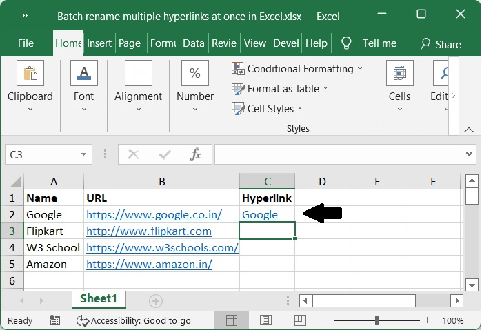
Step 3

To apply this formula, press the Enter key on your keyboard and then move the auto fill handle over the cells. As shown in the below screenshot.

Conclusion

In this tutorial, we explained in detail how one can Batch rename multiple hyperlinks at once in Excel.